Heyy everyone! Welcome to this blog on gradient descent, and various features and calculations in it.

What is gradient descent?

If you're not familiar with it, Gradient descent is a ML optimization algorithm, that helps finding a local minimum of a differentiable function really effectively.

It's super popular, and used it most cases when doing any kind of training, testing, or learning.

Let's get started with gradient descent!

Why is it called gradient descent?

When you have 2 or more deriatives of a function, it's called gradient. And when those deriatives reach the lowest or the optimal point, also called descend using loss function, that's when it becomes Gradient Descent!

It's an effective way of reaching the local minimum of the function, which is the most appropriate value for the pattern prediction.

It basically takes a random input parameter, starts by calculating the error, uses the minima algorithm to minimize the error, and keeps on repeating that until the lowest minimum is found.

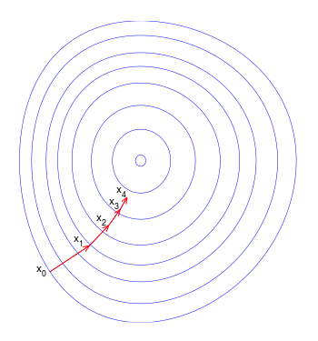
This is the layered data, which is passed to the algorithm. The pointer of the gradient descent starts to calculate the points, and uses the algorithm below to keep changing values faster in the start and slowing down in the end so It can find the perfect point to get the prediction for. This is how it works.

Gradient descent has it's applications almost everywhere, including softmax algorithms used in deep learning layers, for example: tf.keras.layers.Dense(100, activation="softmax"). It's preferred the most due to it's fascinating way of getting best predictions, and the efficiency it gives when running the ML model training. Gradient descent isn't just limited to certain types too, It can calculate for linear and non-linear data, hence making it suitable for working.

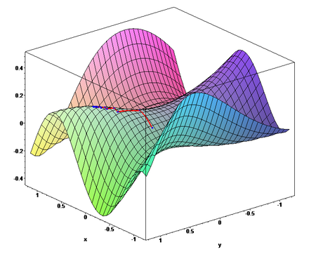
This is how the Gradient descent 3D representation looks like. It forms a surface area for search in start, and slowly narrows down as it goes, so It takes small steps and gets the perfect spot to stop.

The algorithm used for calculating error, and making it better

The equation is Prediction = intercept + slope * given_value

So, Slope is the angle of the straight line, which is going through the points for finding the prediction for the given value and the intercept is the value of the linear predictor when all covariates are zero.

The gradient descent algo converging into the local minimum is also guaranteed, but not the best thing. We need the global minimum, the smalled point all over the graph which is the perfect spot. But sometimes local minima can be global minima, under the convex funcrion, where it converges into the best soution.

In linear regression, this is the line of best fit or best value.

Calculating STEP size and getting better parameters

When we want to calculate the step size for the prediction and substitution, we use this: Slope (the angle of the line) * Learning rate (the rate for descending.)

And getting a new intercept for better prediction:

New and better intercept = the old intercept - newly calculated step size.

We moved a lot towards the optimal result after changing the step, which is what we need.

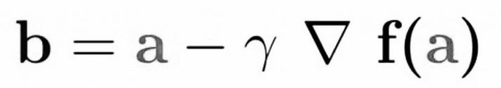
Explanation of this: b is the next position of the algorithm, while a represents the current position. The minus sign refers to the minimization part of gradient descent. The gamma in the middle is a waiting factor and the gradient term (Δf(a)) is simply the direction of the steepest descent.

Types of gradient descent

Stochastic Gradient Descent

It's an type of gradient descent, which is really efficient. When we have a million points and not enough resource and time to calculate, that's when stochastic GD comes into play. It swiftly jumps randomly until it finds the best value hence fast and good.

The random jumps can be expensive though than batch gradient descent. Usually the frequency results in noisy gradients, that may cause the error rate to be randomized instead of being optimized and descent.

Batch Gradient Descent

Batch gradient descent calculates the error for each example within the training dataset, but only after all training examples have been evaluated does the model get updated. This whole process is like a cycle and it's called a training epoch.

Advantages:

• Stable gradient
• Stable convergence
• Stable error measure

But the worst thing about this algorithm is it requires the entire training dataset be in memory / memcached and available to the algorithm while training.

Mini-Batch Gradient Descent

Mini batch gradient descent is a better method since it utilizes both SGD and Batch GD. It breaks the dataset into pieces to make it efficient using CPU cores, and performs update for each batch. It hence implements a robust and efficient result inheriting from the previous algorithm.

Mini-batch gradient descent is a variation of the gradient descent algorithm that splits the training dataset into small batches that are used to calculate model error and update model coefficients.

Why is it the best:

• It always finds the global minima easily.
• The batches are split and are robust hence works swiftly
• The batching allows both the efficiency of not having all training data in memory and algorithm implementations.

I hope this was informative article on Gradient descent and working. Time for me to go, See you next time!