Writing our first deep learning model
Creating a simple model to classify images of clothing using Tensorflow and Python

16 y/o engineer from India.
Feel free to drop me a mail, or get in touch through my socials! 👋
Hey everyone! In this article, we're gonna be writing our first deep learning model from scratch. We'll be covering the basic things with explanations on the way, and then do our model that predicts and then export it for normal use.
We'll be using Google colab, An awesome jupyter notebook by google with Free GPU, specially made for ML.
Without any further ado, Lets dive into it!
Creating our first notebook
When you first visit the link, It will prompt you for login, if you're not logged in to google, then a prompt appears where you can select one of the previous notebooks you have or create one. Select create a new one, and rename it.
Here is how you can do it,
Starting with imports and data loading
We'll be starting with fashion MNIST dataset, a dataset containing images of clothing, over 70000 samples with pixel size of 28x28, consisting of 10 categories of clothing.
![]()
Let's start off by first configuring colab to use tensorflow version 2.x which is the latest one.

When you type in a cell, you need to hit run to run the code and go to the next, a really awesome way of running and visualizing code.
Once done, we're ready to import the modules we need to get started.
import tensorflow as tf
from tensorflow import keras

# Helper libraries
import numpy as np
import matplotlib.pyplot as plt

print(tf.__version__)
When these are done, we can load the datasets safely. Use the following codeblock to do it.
data = keras.datasets.fashion_mnist
This loads the Fashion MNIST dataset class into the variable data, which needs to be invoked to get the actual numpy arrays containing the data.
It can be loaded by invoking in this following way:
(train_images, train_labels), (test_images, test_labels) = data.load_data()
This segregates the images also into tuples, ready to be used.
Time to define the clothing categories. Reading the documentation at tensorflow.org, you get that there are 10 categories, which are the following. Define them accordingly.
class_names = [
    "T-shirt/top", "Trouser", "Pullover", "Dress", "Coat"
    "Sandal", "Shirt", "Sneaker", "Bag", "Ankle boot"
]
Now, it's time to clean the data. Computers understand values between 0 and 1, that is binary. The pixel values in the dataset is given as the range of 0 - 255, which isn't understandable. We need to bring them into the range of 0 and 1 by preprocessing it. To examine the data using colormap first, here's how to do it.
# Create a figure
plt.figure()

# Display an image
plt.imshow(train_images[0])

# Enable colorbar and disable grid
plt.colorbar()
plt.grid(False)

# Show the plot
plt.show()
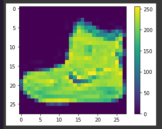
If you inspect the first image in the training set, you will see that the pixel values fall in the range of 0 to 255. Now time to preprocess in the correct range.
Do this to preprocess and change the range into 0 to 1.
train_images = train_images / 255.0

test_images = test_images / 255.0
Now you can examine the data my displaying it using Matplotlib cmap. Let's make a range of data using subplots to examine them.
plt.figure(figsize=(10, 10))

for i in range(25):
    plt.subplot(5, 5, i+1)
    plt.xticks([])
    plt.yticks([])
    plt.grid(False)
    plt.imshow(train_images[i], cmap=plt.cm.binary)
    plt.xlabel(class_names[train_labels[i]])

plt.show()
This shows us the visuals and the labels of the clothing type like this:
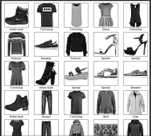
Great! We have successfully pre-processed out data, Time to prepare and train our model.
Creating a model
We have pre-processed our data, Time to create the models.
But before that, we need to understand the data. We saw that the pixel count is 28 by 28, that is in the following form:
[
    [0.3, 0.8, 0, ...]
    .
    .
    .
    [1, 0.2, 0.7, ...]
]
Which is a matrix of 2 dimensions. We need to flatten it and make it a 1D array of pixels. Lucky for us, there's already a Flatten layer in Keras that flattens the data for us. Let's start by building the model.
model = keras.Sequential([
    keras.layers.Flatten(input_shape=(28, 28)),
    keras.layers.Dense(128, activation="relu"),
    keras.layers.Dense(10, activation="softmax")
])
Let's understand it.
- The first layer get's an input of 2D, 28 by 28 size, hence we define as
(28, 28)and pass it to the Flatten layer. - Once done, we make a dense layer of size 128, enough to fit our data and process it.
- And finally the last layer, which is a Dense layer of size 10, It's sized 10, as we have 10 categories of clothing.
- The activation is relu in second one for faster and better processing, The formulae is
y = max(0,x), It stands for rectified linear unit. - And softmax for the last one since we're classifying. Softmax is used as the activation function for multi-class classification problems where class membership is required on more than two class labels.
Once done, you can take a summary of the model by using model.summary()
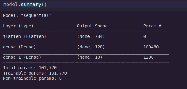
Looks great, Now we need to compile our model.
Here's how to do it:
model.compile(optimizer="adam", loss="sparse_categorical_crossentropy", metrics=["accuracy"])
Here, the optimizer is the important section that affects how good our model will be, We used adam, as it's pretty popular and awesome. The loss function is the one, that calculates where our model goes wrong, and Sparse categorical crossentropy is a pretty awesome one, and metrics set to a list with just accuracy, since we need how good our model performs.
Now, once it's compiled, we need to fit our data and train it.
Here's how to do it:
model.fit(train_images, train_labels, epochs=10)
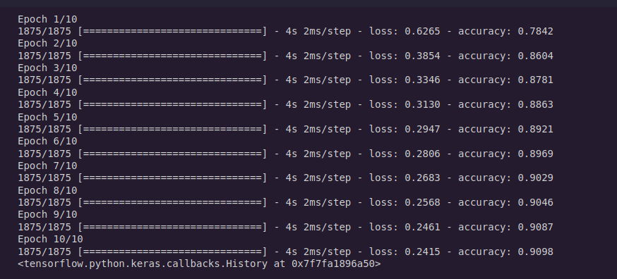
Here, epoch is the count of number of batch the model sees randomly, and learns from it. Like a batch is broken into 10 pieces, 9 is used for training and last one for testing and improving it, It's repeated 10 times too.
It's gonna start a long output, time for a coffee break! Once you're done, it's the moment of truth how good the model is gonna perform.
Testing the model
Testing isn't really hard, in fact it's really simple.
It can be done in a single step.
test_loss, test_acc = model.evaluate(test_images, test_labels, verbose=2)
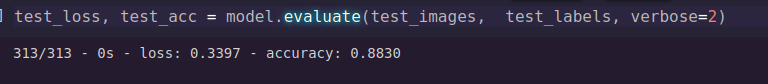
We evaluate the model now on the test set we had, and then grab the loss and accuracy, Bam, we are done!
Now you can get the accuracy and print it, print(f"Accuracy: {test_acc}")
And you're done with an awesome model.
Time to now export the model :)
Here's how you can do it real quick:
model.save("/content/MyAwesomeModel.h5")
And it'll be saved as the name specified, in your google drive.
Summing up!
Time to wrap things up and just re-call what we just did.
Here are the steps to create an amazing model. We don't have a perfect model, because of not enough training, hyperparameter tuning and layer configuration. These are some of the factors.
- Get the data
- Clean the data
- Make the data to be computer readable.
- Create the model
- Compile it after supplying a optimizer, loss function and metrics to the compile function
- Fit the model with the training data, and add the epoch count.
- After training, evalute it!
- Boom, you get the accuracy :)
Important links
You have reached the end. Thank you so much for reading this article, I hope you loved it, and learnt something awesome! If you have any queries or feedback, Hit me up in my twitter handle 👋 Let me know what you think of this blog! 👀
Let's connect 🌟
→ Github
Catch you next time ✨


